Common metrics for ESUs
Multivariate dynamic linear modeling (DLM) was used to estimate population specific mean trends in each ESU from the log of total spawner counts. The result is an estimate of the mean or smoothed total spawner counts, from which summary statistics regarding trends were computed. In addition, a univariate DLM was applied to the logit of the fraction wild estimate to produce a smoothed fraction wild time series. This was used to produce an estimate of the mean wild spawners (for years when fraction wild estimates were available).
The mean or smoothed total spawner count is similar (in concept) to a 3- or 5-year geometric mean; the goal is the same—to produce an estimate that smooths over single year variation. The multivariate DLM approach has a number of advantages. Most importantly it is a statistical model for which maximum-likelihood diagnostics, model selection criteria, and confidence intervals are available. It is a time-series model, which addresses temporal autocorrelation in the data. It deals with missing data and provides an estimate for the missing year with appropriately wider confidence intervals. And lastly, it allows us to use information across all populations within an ESU to estimate the level of year-to-year trend variation—the process variance—and allows us to estimate the covariance, which is often high, across populations. The latter improves estimation of missing values because populations with data in one year help inform the values for populations with missing data that year.
Dynamic linear modeling for time-varying trend estimation
Dynamic linear models (DLMs) are similar to linear regression models with a yearly trend. Like a classic trend analysis using linear regression, the goal is to estimate the smoothed spawner count at , where is year (time). Linear regression models, however, use a time-constant yearly trend while DLMs allow the trend to be time-varying.
A classic linear regression of log spawners () against year treats the trend () or yearly growth in the smoothed spawner count as a constant and fits the following model: where are the observations, is the mean of and are normal-distributed errors. The smoothed spawner count in year is the smoothed spawner count in year plus the constant trend value . Normally we write this model in classic linear regression form as with . A DLM, in contrast, allows us to fit a model with a time-varying . Specifically, the following model The time-varying , , is modeled as , where is the mean of across all and is a normally distributed random variable.
Figure 1 shows some example spawner data where a time-varying sinusoidal (yearly growth rate) was used to generate counts (the circles) using and . This model can also be written . The black line in the top panel of Figure 1 shows the true mean . The red line shows the estimate from a linear regression of against year with a non-time-varying . The blue shows the estimate from a DLM where the is allowed to vary in time. The bottom panel shows the estimate of compared to the true sinusoidal that generated the data. This illustrates the power of DLM when the objective is to estimate a time-varying trend.
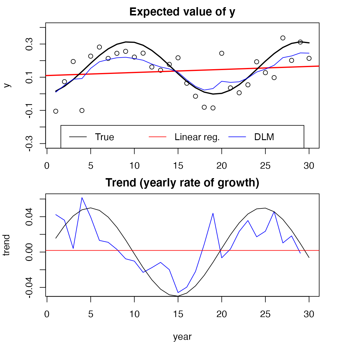
Figure 1. This figure compares a trend analysis using a non-time-varying trend (red) via linear regression versus a trend analysis using a time-varying trend (blue). The black line is the true value and the dots in the top panel are the observations of the black line in the top panel.
Multivariate DLMs for analysis of multiple time series from one ESU
A multivariate DLM allows one to estimate time-varying trends using a set of observed time series, in our case populations within ESU, where parameter sharing is allowed across the time series. Specifically, one can constrain the variances to be the same across time series and to allow covariance across time series. The latter allows information from time series with data in year to help inform the estimate or the smoothed for time series that have no data in year .
Mathematically, the model being fit is The are the mean of , so the average long-term trend and the trend at year is . The and are error terms drawn from a multivariate normal distribution with variance-covariance matrix and respectively. The structure of and allows one to specify different types of parameter constraints (for example equal variances).
Treatment of NAs and 0s
NAs are years with missing spawner counts. The spawner count for these years will be estimated with the DLM and the estimate will take into account the spawner counts in that population both before and after the missing year. The estimate will also take into account the spawner counts for that year in the other populations and the degree to which populations within the ESU are temporally correlated.
The modeling uses log-spawners and 0s in the counts will be replaced with NA (log(0)=NA). This will have minimal effect if 0s are rare, but if 0s are common, then caution is required since removal of 0s will bias the estimates upward. For the raw metrics, such raw geomeans, the 0s are also replaced with NA. Thus when a 0 appears in the 5-year range used for a geomean calculation, that year is replaced with NA and only the remaining 4 years are used to compute the geomean, i.e. the reported raw geomean would be the product of the 4 non-zero counts raised to the 1/4 power.
Model selection
Model selection was used to select the structure of and . The following structures were explored for : diagonal with unequal variances (no covariance), diagonal with equal variances, one variance and one covariance across all populations, equal variances and covariances across similar run timings in a population, and unconstrained (unique variances and covariances across all populations). For the following structures were explored: diagonal with unequal variances (no covariance) and diagonal with equal variances. The represents the residual variance, non-time-dependent error and was assumed not to covary across populations ( and cannot both have covariance terms in the DLM due to identifiability constraints). Across the majority of ESUs, model selection gave the most data support (quantified with AICc) to a with one variance and one covariance across all populations in an ESU and a with one residual variance across populations.
Code to fit a multivariate DLM
The MARSS R package was used to fit multivariate DLMs to the log-spawner counts (or indices in some cases). The package handles missing data entered as NAs for missing years. The following example code shows how to fit two time-series via a multivariate DLM using the MARSS R package.
library(MARSS)
logspawners = log(matrix(
  c(
1106, 1503, 853, 566, 251, 424, 783, 639, 566, 413, 1035, 890,
7348, 6880, 2699, 1096, NA, NA, NA, 1318, 1127, 472, 637, 869
), 2,12, byrow=TRUE))
model=list(
  Q="equalvarcov",
  R="diagonal and equal",
  U="unequal")
fit=MARSS(logspawners, model=model)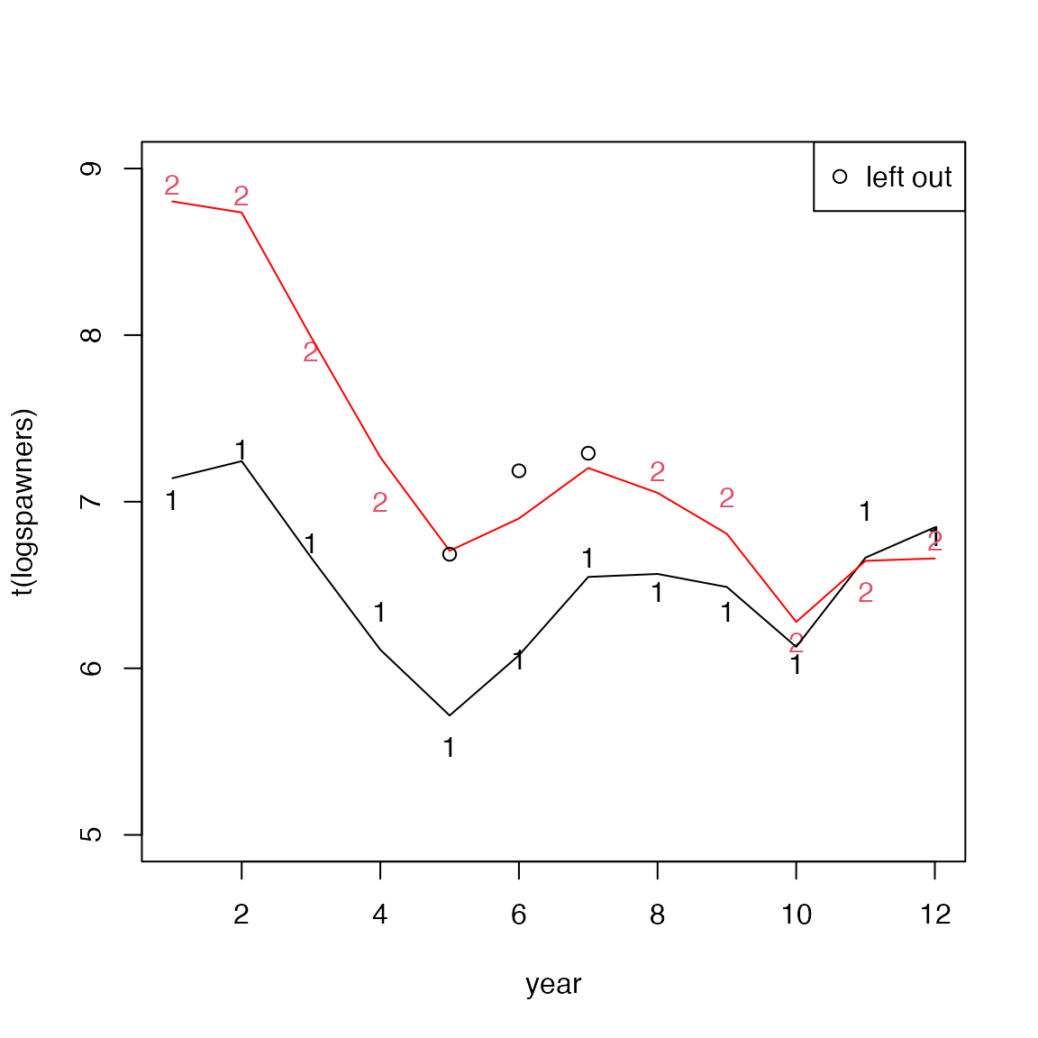
Figure 2. The estimated smoothed log-spawners using a multivariate DLM. Notice that the information from the early years when data are available for time-series 1 are used to inform the estimate for time-series 2. In the ESU reports, these estimates are shown in light grey. Because the model works in log-space, raw spawner counts that are equal to 0 are replaced with NA (log(0)=NA). If there are few 0s in the data, this will only slightly affect the estimates but if there are many 0s in the data, caution is required since removal of 0s will bias the estimates upward.
Wild spawner and fraction wild estimates
For some populations, there were fraction wild estimates. However, for many populations, these data were noisy and had many missing years. In addition, the number of years with fraction wild information was often shorter than the years with total spawner counts. To estimate a smoothed wild spawner estimate, similar to the smoothed total spawner estimate, the smoothed total spawner estimate was multiplied a smoothed estimate of the fraction wild. The smoothed estimate was produced by fitting a univariate DLM to the logit of the fraction wild estimates. with a time-varying . Specifically, the following model The smoothed wild spawner estimate at time was then . Each fraction natural origin time series from an ESU was fit independently (no covariance assumed across populations). The fraction wild estimates were only extended 1 year before and 1 year after the last fraction wild data points (the observed data).
Summary statistics
The following summary statistics were reported for the smoothed total spawner estimates, the smoothed wild spawner estimates, and the raw total and wild spawner estimates.
- 15 year trends A linear regression was fit to 15 years of the mean wild spawner estimate and the slope (trend) reported.
- 5 year geometric means 5-year geometric means were computed from the mean wild and total spawner estimates and the raw total and wild spawner estimates. Note 1 the mean estimates have no missing values. The raw estimates may have missing values. When there were missing values, the geometric mean was computed from only from the non-missing values. For example, if 3 values were available, was reported. Note 2 0s in the raw data are replaced with NA thus the raw geomean is the geomean only from the non-zero counts.
- average fraction wild These were computed from the raw fraction wild estimates. Os in the raw data were left in (not removed). NAs were treated as NAs (did not affect the estimate).
- productivity metric Because age of return data was not consistent nor available across ESUs and populations, a generic productivity metric was computed as the mean wild spawner estimate at year divided by the mean total spawner estimate at year for Coho and for all other species.